This note is especially for beginners.

Maybe you need to pick up "some" basic "mathematics" rather quickly.
So really..., my emphasis is on "rather quickly".

So, I am really not sure of it, but I hope that this note can be of use.
Ofcourse, I hope you like my "style" and try the note anyway.

1. Introduction to the "derivative function".

1.1 taking the "Limit" of a function for a certain "x"

Before we go discussing "differentials" I need to touch on the subject of "taking the limit". This is really easy to understand.

Professional mathematics can be very "formal" and can be quite hard to read, even if the subject is realtively easy.

Ofcourse I fully understand that the professional literature, is way way way better than my notes, but my goal simply is,
that you grasp concepts quickly...

Suppose you have the well-behaved function f(x)=2x+3.

Now, if you want to know the value of f(x), for say x=3, then you simply fill in "3" into "f(x)" and calculate "2x3 + 3 = 9"
Here, it is easily done, since "f(x)=3x+2" is a smooth continuous function (no gaps, no asymptotic behaviour).

You may also say this: if "x" approaches "3" very closely, then to what "y" will f(x) go to? In the example above,
f(x) will ofcourse neatly approach 9, if "x" approaches "3".

Sometimes mathematicians also write it as:

lim_x-->3 2x+3 = 9

However, when you have a function which is "not neat", or not defined, for a certain x, the "lim" notation will help to correctly
decsribe f(x) for that "x".

Suppose we have the function "f(x)=1/x". This function behaves rather nicely, except when "x" approaches '0'.
In the figure below, you see a graph of "f(x)=1/x". We have not dealt with such functions before. But here, I only
use it to illustrate something that is called "asymptotic behaviour".

When "x" gets very large (positive or negative), then "y" simply slowly approaches 0, and that's all fine,
from a mathematical point of view.

But, when "x" approaches "0", we run into problems, since mathematically, "1/0" is not defined.
It's mathematically "not nice" to say: "f(0)", since division by zero is not defined (actually, it runs to infinity).

Figure 1. f(x)=1/x



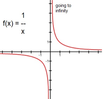
If x approaches '0' from the postive x-axis side, then "y" goes to + infinity.
If x approaches '0' from the negative x-axis side, then "y" goes to - infinity.

But, in the "limit" notation, it looks way better:

lim_{x ↓ 0} 1/x --> infinity

lim_{x ↑ 0} 1/x --> -infinity

So, we are not saying "x" equals '0', but we say instead that "x" approaches '0'.

But, for a nice, continuous functions, the "lim" notation simply means the value of f(x), for a certain x.
Nothing special here !
That is, say that for a nice, continuous function, that "x" approaches "a", then:

lim_x-->a f(x) = f(a)

We will mainly use this "normal" behaviour, instead of approaching "gaps" or asymptotes etc..

Please note that for any smooth continuous function f(x), it holds that:

lim_h-->0 f(x + h) --> f(x)

Since, if h really is extremely small, then "x+h" is practically the same as "x", and f(x + h) is practically the same as f(x).

1.2 Introducing Δf(x)/Δx

We have already seen some functions, for which holds that each "x" is mapped to one "y".
Think for example of a linear equation, y=ax + b, where that condition is certainly true.

But it's true too, for a quadratic equation like y=ax² + bx + c, or, for polynomials in general.

We always have silently assumed (so to speak), that "functions" are rather "smooth" too, meaning that there
are no "gaps", and there (usually) is no "asymptotic behaviour" in the sense that the function very quickly "runs"
to infinity. For an example of the latter one: you might take a look at the tangent function (tan(x)), discussed in note 4,
which shows such asymptotic behaviour when x gets near π/2.

A function which does not have such irregularities, like gaps, is often characterized as "a continuous function".

When we have an equation like "y=x³ - x", we also often say that y=f(x),
where the function "f(x)" then is the same as "x³ - x".

It's just important, especially in this note, to get used to the notation y=f(x), where f(x) can be any
sort of function.

Question: suppose we have the equation y=ax+b, then what would be f(x)?
Answer: f(x)=ax+b

What could be called a "core" idea of taking the differential of a function?

The text taking the differential already says a bit what we are looking for.

We essentially want to find the rate of change of "y", which is the same as "f(x)", compared to the
the rate of change of "x".

Or: we want to find the "ratio" of the change of "f(x)", to the change of "x".

Does this give us extra information? Yes, it does. Take a look at figure 2 below.

Figure 2.



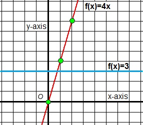
Case 1. We see a blue line, "f(x)=3", which is constant. No matter at which "x" you are, "y" will always be "3".
Does this function posess any sort of "rate of change"? No. f(x) never changes so the rate of change=0.

We might express the change of f(x) as Δf(x), and the change of x as Δx. Indeed, "Δ" is a
universal symbol for "delta", meaning "change".

In the case of the constant line f(x)=3, the ratio would be Δf(x)/Δx, and that is "0", since
Δf(x) is "0". The line is constant, so there is no change at all.

Case 2. We also see the red line "f(x)=4x". So, if you change "x" by one, the change of y will always be four times as large.
Really. For example, if you are at x=0, and take 5 steps to the right, then you are at x=5 on the x-axis.
However, y=f(5)=20. So, x changed by 5, and the value of y changed by 20.

But you could also have considered a small change in "x". Suppose, on the x-axis, you are at x=1.
Next, you go to x=1.1 (so the change is only "0.1"). The corresponding change in f(x) would then be "0.4".

In this case (of f(x)=4x), you might decide that Δf(x)/Δx =4.
No matter what change in "x" you would consider, then the corresponding change in "f(x)" is 4 times as large.
You might say: alright, but wasn't it already "evident" in the function itself: y=4x ? True.

In general, the ratio of the changes might be expressed as:

ratio of the rate of change=

Δf(x) ------ Δx

(equation 1)

I would like to re-write that a bit.

A: If we would change "x" to "x+h", where "h" can be any value, then the change in x would be "h". That's evident.

B: For the corresponding change in f(x), we can say that it has to be "f(x+h)" minus "f(x)".

For the statement(B), we may not say that de difference in the function is "f(h)". Why not?
Well, above we have only considered simple lines. But suppose the function is a parabola.
In such a case, depending on where you are on the x-axis, the value of f(h) varies enormously.
We always need to consider the change of x, with a truly corresponding change of f(x).

It means: you can always "pick" any "x" to start with, say a certain "x" denoted by "x₁",
and then change "x₁" to "x₁+h".
But then we always have to consider the change in the values of "f(x₁+h)" and "f(x₁)",
thus with respect to that particular "x₁".

In general, the ratio of the changes might thus be expressed as:

ratio of the rate of change=

f(x + h) - f(x) ----------------         h

(equation 2)

In considering the ratio of changes as we have seen in the examples above, does it add to our knowledge?

With the actual functions (the lines) that we have seen sofar (y=3 and y=4x), the addition in knowledge is not really great.
Ofcourse, when the ratio is "0", you can say that we thus deal with a line with a constant value.
And, when the ratio is "4" all the time (for every x), we can say that we thus deal with a line that always
"changes" 4 times as fast as "x".

But it gets more impressive if we consider more complicated function. Let's study a a good example in chapter 3.

1.3 The differential of a function, and the "derivative" function, of a function.

I hope you can see the following reasoning, with the aid of figure 3.

If the difference between x and x+h is small, and thus also the difference between f(x) and f(x+h) is small too,
we can draw a straight line between those two points on the curve of f(x).
Note that this line is almost a "tangent-line', for that small neighborhood.

In the example shown in figure 3, I arbitrarily choose for the function f(x)=x², but it could have been
any continuous function.

Figure 3. Tangent line, if "h" gets small.



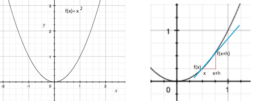
If h is really get very small, the line is going te become the "tangent line", with a "gradient" (or slope),
which is very much the same as the gradient of f(x) for that local neighborhood.

So, if "h" getting very, very small, we more and more end up with a true tangent line.

So, let's try to calculate the "differential" (as was shown above), when h -> 0:

lim h-->0

f(x + h) - f(x) ----------------         h

=>

lim h-->0

(x + h)2 - x2 ----------------         h

=>

lim h-->0

x2 +2xh +h2 - x2 ----------------         h

the x² and - x², will cancel each out, so we have:

lim h-->0

2xh +h2 --------     h

This is the same as:

lim h-->0

2xh/h +h2/h

= 2x

We have "2x", since 2xh/h - h²/h = 2x -h, and, because h approaches '0', we thus end up with 2x.

Mind you, we have a great result here. We did not made any assumptions on "x" itself, so
the derivation is valid for the whole of the "x-axis", thus for complete f(x).

What we found is that for the function f(x)=x², the gradient of tangent line at any "x",
is "2x".

-So, if you want to know the gradient of the tangent line for, for example x=3, then that would be "6".
Thus, the tangent line itself would be parallel g(x)=6x.

-And, if you want to know the gradient of the tangent line for, for example x=5, then that would be "10".
Thus, the tangent line itself would be parallel to g(x)=10x.

-And, if you want to know the gradient of the tangent line for, for example x=8, then that would be "16".
Thus, the tangent line itself would be parallel to g(x)=16x.

Indeed, the slope is getting steeper if "x" increases, as expected with this parabola.
In chapter 3 we will explore tangent lines further in detail.

At this moment, it's important to understand that the derivative function of f(x)=x²,
turned out to be g(x)=2x. This itself is just an ordinary function.

Here I only use "f" and "g" to be able to explicitly distinguish both functions.
But there already exists a way to denote both functions in a proper manner.
Most mathematicians have agreed to use this.

If f(x) is the function, then the derivative function is notated by f '(x)

Please note the ' symbol, to denote the derivative function.

In physics, and some other sciences, the "d/dx" (or "∂ / ∂ x") is also often used:

f '(x)=

df(x) ---- dx

(equation 3)

Actually, often the "∂" symbol is used for functions having more than one variable, like f(x,y,x).
For functions depending on just one variable, like f(x), simply the letter "d" is used, which then leads to the d/dx notation.

Note that equation 3, is actually the "infinitesemal" variant of equation 1, where Δx goes to "dx".

Then read it as follows: we want to see the change of f(x) (the delta), compared to (as a ratio to)
the corresponding change of "x" (also a delta), whereas the delta is assumed to approach zero.

As said before, we will often use the "f '(x)" notation, to denote the derivative function.

2. Methods for finding the derivative function.

Above we found that f '(x)=2x, is the derivative function for the parabola f(x)=x².

For many types of functions (like e.g. x³ and higer degree, sin(x), etc..) it can be proven how to obtain
the derivative function. We have seen one example on how to do that, and really, all others go in a similar way.
So, we are not going to prove the method on how to obtain the derivative function for all those type.
And, it's really not neccessary.

1. The derivative of a Linear equation:

Here, we know that f(x)=ax+b

(1): Let's start with the simplest case: f(x)=c, or, what is the same, y=c, where "c" is some constant number.
So this is a "constant line" running parallel to the x-axis. It has no gradient (or slope),
and it does not change at all if "x" changes. See figure 1 for an example of y=c.
Since it has no gradient, we have:

f(x)=c

then

f '(x)=0

(2); In case of general linear function, we can say that it has a certain slope, ot gradient. This gradient is constant,
since the function is a line. Per definition, a line has a constant slope, isn't it?
So, here is how to obtain the derivative function:

If:

f(x)=ax+b

then

f '(x)=a

or in the d/dx notation:

d ax+b -------- dx

= a

Yes, indeed! The coefficient "a" determines the "angle" of that line with the x-axis, or in other words: it's gradient.

In a way, we may say that a line is it's "own tangent line".

Example:

f(x)=3x+2
f '(x)=3

This means that the line 3x+2 has a gradient of "3", meaning that for each single step of "x", then "y" climbs 3 steps up.

Example:

f(x)= -4x-6
f '(x)= -4

Note the "-" signs. This means that the line -4x-6 has a gradient of -4, meaning that for each single step of "x",
then "y" sinks 4 steps down.

2. The derivative of a polynomial of any degree:

Suppose we have the function:

f(x) = axⁿ (where a is some constant number).

The power "n" can be any integer, like n=3, or n=4 etc... Suppose we have n=3, then the function would be f(x) = ax³

Then, using the method demonstrated in section 1.3, it can be proven that the derivative function is:

If f(x) = axⁿ

then:

f '(x) = an x^n-1

or in the d/dx notation:

d axn ------ dx

= an xn-1

Example:

f(x)= 4 x³

then

f '(x)= 12 x²

Example:

f(x)= x²

then

f '(x)= 2 x

yes, this latter example we have derived ourselves in section 1.3.

3. The derivative of a "sum" of functions:

What we mean is this: suppose we have f(x) + g(x).
Or if you like, suppose we have the function v(x) for which holds: v(x) = f(x) + g(x).

Then how do we determine derivative function of v(x)?

That's really simple: it's like this:

If:

v(x) = f(x) + g(x)

then

v '(x) = f '(x) + g '(x)

So, simply find the individual derivative function, of each part of the sum.

Example:

f(x) = 3 x⁴ + 2 x²

then

f(x) = 12 x³ + 4 x

Example:

f(x) = -2 x² + 2x

then

f '(x) = -4 x + 2

4. The derivative of a "product" of functions:

Quite similar to (3), but this time we can write that v(x) = f(x) . g(x)

Then how do we determine derivative function of v(x)?

If:

v(x) = f(x) g(x)

then

v '(x)= f '(x) g(x) + f(x) g '(x)

Example:

f(x) = 2x² . 2 x³

then

f '(x) = 4x . 2 x³ + 2x² . 6x² = 8 x⁴ + 12 x⁴ = 20 x⁴

5. The "chain" rule:

Suppose we have a function that can be viewed as:

f(x)=u(v(x))

So, we first have "v" operating on "x", then followed by "u" operating on "v(x)".

This is not uncommon. Just think of for example f(x)=(x²-3)³

So, we can interpret it as: u=v³, while v=x²-3.

It has been proven that:

If f(x)= u(v(x)) then

f '(x) = u '(v(x)) . v '(x)

Example:

Suppose we have:

f(x)=(2x-3)⁵

If we treat it like this:

v=(2x-3)
u=v⁵

Then using the upper rule, we find:

f '(x) = 5(2x - 3)⁴ . 2 = 10(2x - 3)⁴

6. The derivatives of sin(x) and cos(x):

The sin(x) and cos(x) functions are very important in math and science in general.

Using the method demonstrated in section 1.3, it can be shown that:

If f(x)=sin(x) then f '(x)=cos(x)

If f(x)=cos(x) yhen f '(x)= -sin(x)

7. The derivatives of sinⁿ(x) and cosⁿ(x):

Thanks to subsection 6, we know what the derivatives of sin(x) and cos(x) are.

But what are the derivatives of sinⁿ(x) and cosⁿ(x), where "n" is some power.
For example, if n=2, we would have sin²(x) and cos²(x).

In all this sort of tasks of finding the derivatives, the chain rule must be used.

Suppose we want to find the derivative of y = cos²(x).

Let u = cos x, so that y = u²

Thus y = (cos(x))² = f(g(x)).

According to the chainrule:

[f(g(x))]' = f'(g(x))g'(x)

thus, if we exactly follow the chain rule:

[f(g(x))]' = -2cos(x)sin(x).

8. The derivatives of sin(xⁿ):

For the cos variant, the argument goes the same way as shown below.

Let's consider the situation where we need to find the derivative of sin(x²).
For higher powers, the method is exactly similar to the method below.

We need to use the "chain rule" of subsection 5.

Let f(u) = sin(u) and g(x) = x².

Thus y = sin(x²) = f(g(x)).

According to the chainrule:

[f(g(x))]' = f'(g(x))g'(x)

thus, if we exactly follow the chain rule:

[f(g(x))]' = cos(x²)(2x) = 2xcos(x²).

9. The Quotient rule

Suppose we have:

f(x) =

g(x) ---- h(x)

Then f '(x) is:

g '(x)h(x) - g(x)h '(x) ----------------------         (h(x))2

3. The second derivative.

If we have f(x), then usually (except at gaps, asymptotes etc..), we can determine f '(x), or the derivative function.

However, in general, we can also determine the derivative function of that derivative function.

I mean, you might also say that f '(x) is the first derivative function.
But if f '(x) itself can be differentiated, then we may obtain the second derivative function f "(x) of f(x).

Example:

Suppose f(x)= 2 x³ + 3x.

Then:

f '(x) = 6x² + 3

And

f "(x) = 12x

We know that the first derivative is interpreted as the "gradient" (or slope) of the tangent line at f(x).

The second derivative, may be interpreted as the "gradient" (or slope) of the tangent line at f '(x).

Or, if we want to see that in the "d/dx" notation:

f "(x)=

d2 f(x) ------ dx2

What we have seen in this note is not the whole story, but for this note, it's quite enough.
I want my notes to be "fast", but not overwhelming....
It's way better to let the material of this note "sink in", and try some examples by yourself.

4. Some further examples.

f(x) = a^x -> f '(x) = a^x ln(a) (a>0)

f(x) = a^g(x) -> f '(x) = ln(a) . g '(x) . a^g(x)

f(x) = ln(x) -> f '(x) = 1/x

f(x) = ln(ax) = ln(a) + ln(x) -> f '(x) = 1/x

f(x) = ^alog(x) -> f '(x) = 1/xln(a) (a>0)

f(x) = sin(x) -> f '(x) = cos(x)

f(x) = sin(ax+b) -> f '(x) = a.cos(ax+b)

f(x) = cos(x) -> f '(x) = -sin(x)

f(x) = cos(ax+b) -> f '(x) = -a.sin(ax+b)

f(x) = tan(x) -> f '(x) = 1/(cos(x))²   or: (tan(x))² + 1

f(x) = e^x -> f '(x) = e^x

f(x) = e^g(x) -> f '(x) = g '(x) e^g(x)

5. How to analyze, or "investigate", a function.

In note 6, I will collect all theory needed to (what mathematicians call) analyze a function, by using
a good illustrative example.

Here I mean, for example, how to find the intersection(s) with the x-axis, the intersection with the y-axis,
and "special points", like the "minima" and "maxima" of that function.

For about those special points: we know that if the gradient is '0', then the tangent line is parallel
to the x-axis, and it must be on a "hill" (maximum), or "crest" (minimum). Only at such point, the gradient (or slope) is then '0'.

So: How to analyze a function? Please see note 6.

That's it ! Hope you liked it.

The next note is a super quick intro in how to "analyze" a function.